Duration 6:11
Don't you have Xlookup Use Index Match Vlookup doesn't works here
Published 13 Aug 2023
In this Excel video tutorial, we are going to learn how to use the Index & Match function in Excel when we can't use the Excel Vlookup function and Excel Xlookup function. These functions are called search functions in Excel, lookup functions. They can automate repetitive processes and repetitive tasks. Just imagine that you have a sales list where you need to fill in the costs of the products, however, instead of checking product by product in another spreadsheet where you have the cost table, it is much easier to use a search function. That way, you don't have to look around, Excel will do the work for you. This is a great way to save time in your daily life and in the job market with Excel, by automating repetitive tasks and processes. The vlookup function can be used when you need to find items in a table or a range by row. For example, you need to look up the price of an automotive part by part number, or find an employee name based on the employee ID. However, vlookup has an error in Excel. It only returns values that are to the right of the reference column, so if you need to return a value that is to the left of the reference column, vlookup does not work. We can then use the procx function or index with corresponding. The xlookup function can be used when you need to find things in rows of a table or range. For example, when looking up the price of an automotive part by part number or finding an employee name based on the employee ID. With xlookup, you can search a column for a search term and return a result from the same row in another column, regardless of whether the return column is on the right or left side of the reference column. The INDEX function returns a value or a reference to a value from within a table or range, that is, it returns the value of an element in a table or matrix, selected by row and column number indices. The MATCH function searches a range of cells for a specified item and returns the relative position of that item within the range. As an example, if the range A1:A3 contains the values 10, 20, and 30, the formula =MATCH(20,A1:A3,0) will return the number 2, because the number 20 is the second item in the selected range. Now that we know how to use the functions above, we can combine functions in Excel, that is, join two functions within the same cell in Excel. And in this free Excel tutorial, we're going to use the Index & Match Function to replace xlookup. #JopaExcel #Dashboard #Excel
Category
Show more


Comments - 0
Related videos for Don't you have Xlookup Use Index Match Vlookup doesn't works here: